
Region masks#
POP includes a default region mask as a component of the grid information. This is often not super
relevant for analyses. pop_tools provides several alternative region masks; these are demostrated here.
Import packages#
%matplotlib inline
import matplotlib.colors as colors
import matplotlib.pyplot as plt
import numpy as np
import xarray as xr

import pop_tools
Load POP grid as xarray.Dataset#
grid_name = 'POP_gx1v7'

ds = pop_tools.get_grid(grid_name)
ds
Downloading file 'inputdata/ocn/pop/gx1v7/grid/horiz_grid_20010402.ieeer8' from 'https://svn-ccsm-inputdata.cgd.ucar.edu/trunk/inputdata/ocn/pop/gx1v7/grid/horiz_grid_20010402.ieeer8' to '/home/docs/.pop_tools'.
/home/docs/checkouts/readthedocs.org/user_builds/pop-tools/conda/latest/lib/python3.9/site-packages/urllib3/connectionpool.py:1097: InsecureRequestWarning: Unverified HTTPS request is being made to host 'svn-ccsm-inputdata.cgd.ucar.edu'. Adding certificate verification is strongly advised. See: https://urllib3.readthedocs.io/en/latest/advanced-usage.html#tls-warnings
  warnings.warn(
0%| | 0.00/6.88M [00:00<?, ?B/s]
1%|▍ | 82.9k/6.88M [00:00<00:10, 649kB/s]
3%|█ | 198k/6.88M [00:00<00:08, 785kB/s]
5%|█▊ | 312k/6.88M [00:00<00:07, 828kB/s]
6%|██▌ | 442k/6.88M [00:00<00:06, 986kB/s]
8%|███▏ | 558k/6.88M [00:00<00:06, 953kB/s]
10%|███▉ | 706k/6.88M [00:00<00:06, 1.02MB/s]
12%|████▋ | 853k/6.88M [00:00<00:05, 1.14MB/s]
15%|█████▍ | 1.00M/6.88M [00:00<00:05, 1.15MB/s]
17%|██████▎ | 1.18M/6.88M [00:01<00:04, 1.32MB/s]
20%|███████▏ | 1.34M/6.88M [00:01<00:04, 1.31MB/s]
22%|████████▎ | 1.54M/6.88M [00:01<00:03, 1.48MB/s]
25%|█████████▎ | 1.72M/6.88M [00:01<00:03, 1.46MB/s]
28%|██████████▍ | 1.93M/6.88M [00:01<00:03, 1.64MB/s]
31%|███████████▍ | 2.13M/6.88M [00:01<00:02, 1.60MB/s]
34%|████████████▋ | 2.35M/6.88M [00:01<00:02, 1.76MB/s]
37%|█████████████▊ | 2.57M/6.88M [00:01<00:02, 1.76MB/s]
40%|██████████████▉ | 2.79M/6.88M [00:01<00:02, 1.86MB/s]
44%|████████████████▎ | 3.03M/6.88M [00:02<00:01, 2.02MB/s]
48%|█████████████████▌ | 3.28M/6.88M [00:02<00:01, 2.00MB/s]
51%|██████████████████▉ | 3.52M/6.88M [00:02<00:01, 2.12MB/s]
55%|████████████████████▍ | 3.80M/6.88M [00:02<00:01, 2.30MB/s]
59%|█████████████████████▊ | 4.06M/6.88M [00:02<00:01, 2.23MB/s]
63%|███████████████████████▎ | 4.34M/6.88M [00:02<00:01, 2.38MB/s]
67%|████████████████████████▉ | 4.64M/6.88M [00:02<00:00, 2.53MB/s]
71%|██████████████████████████▍ | 4.92M/6.88M [00:02<00:00, 2.43MB/s]
76%|████████████████████████████ | 5.21M/6.88M [00:02<00:00, 2.57MB/s]
80%|█████████████████████████████▊ | 5.54M/6.88M [00:03<00:00, 2.76MB/s]
85%|███████████████████████████████▍ | 5.85M/6.88M [00:03<00:00, 2.67MB/s]
90%|█████████████████████████████████▏ | 6.18M/6.88M [00:03<00:00, 2.83MB/s]
95%|███████████████████████████████████▏ | 6.54M/6.88M [00:03<00:00, 2.84MB/s]
100%|████████████████████████████████████▉| 6.87M/6.88M [00:03<00:00, 2.96MB/s]
0%| | 0.00/6.88M [00:00<?, ?B/s]
100%|█████████████████████████████████████| 6.88M/6.88M [00:00<00:00, 9.20GB/s]
Downloading file 'inputdata/ocn/pop/gx1v7/grid/topography_20161215.ieeei4' from 'https://svn-ccsm-inputdata.cgd.ucar.edu/trunk/inputdata/ocn/pop/gx1v7/grid/topography_20161215.ieeei4' to '/home/docs/.pop_tools'.
/home/docs/checkouts/readthedocs.org/user_builds/pop-tools/conda/latest/lib/python3.9/site-packages/urllib3/connectionpool.py:1097: InsecureRequestWarning: Unverified HTTPS request is being made to host 'svn-ccsm-inputdata.cgd.ucar.edu'. Adding certificate verification is strongly advised. See: https://urllib3.readthedocs.io/en/latest/advanced-usage.html#tls-warnings
  warnings.warn(
0%| | 0.00/492k [00:00<?, ?B/s]
40%|███████████████▋ | 198k/492k [00:00<00:00, 1.49MB/s]
0%| | 0.00/492k [00:00<?, ?B/s]
100%|████████████████████████████████████████| 492k/492k [00:00<00:00, 801MB/s]
Downloading file 'inputdata/ocn/pop/gx1v7/grid/region_mask_20151008.ieeei4' from 'https://svn-ccsm-inputdata.cgd.ucar.edu/trunk/inputdata/ocn/pop/gx1v7/grid/region_mask_20151008.ieeei4' to '/home/docs/.pop_tools'.
/home/docs/checkouts/readthedocs.org/user_builds/pop-tools/conda/latest/lib/python3.9/site-packages/urllib3/connectionpool.py:1097: InsecureRequestWarning: Unverified HTTPS request is being made to host 'svn-ccsm-inputdata.cgd.ucar.edu'. Adding certificate verification is strongly advised. See: https://urllib3.readthedocs.io/en/latest/advanced-usage.html#tls-warnings
  warnings.warn(
0%| | 0.00/492k [00:00<?, ?B/s]
20%|███████▉ | 99.3k/492k [00:00<00:00, 765kB/s]
85%|████████████████████████████████▉ | 416k/492k [00:00<00:00, 2.02MB/s]
0%| | 0.00/492k [00:00<?, ?B/s]
100%|████████████████████████████████████████| 492k/492k [00:00<00:00, 963MB/s]
<xarray.Dataset> Size: 11MB
Dimensions:      (nlat: 384, nlon: 320, z_t: 60, z_w: 60, z_w_bot: 60, nreg: 13)
Coordinates:
  * z_t          (z_t) float64 480B 500.0 1.5e+03 ... 5.125e+05 5.375e+05
  * z_w          (z_w) float64 480B 0.0 1e+03 2e+03 ... 4.75e+05 5e+05 5.25e+05
  * z_w_bot      (z_w_bot) float64 480B 1e+03 2e+03 3e+03 ... 5.25e+05 5.5e+05
  * nreg         (nreg) int64 104B 0 1 2 3 4 5 6 7 8 9 10 11 12
Dimensions without coordinates: nlat, nlon
Data variables: (12/15)
    TLAT         (nlat, nlon) float64 983kB -79.22 -79.22 -79.22 ... 72.19 72.19
    TLONG        (nlat, nlon) float64 983kB 320.6 321.7 322.8 ... 319.4 319.8
    ULAT         (nlat, nlon) float64 983kB -78.95 -78.95 -78.95 ... 72.41 72.41
    ULONG        (nlat, nlon) float64 983kB 321.1 322.3 323.4 ... 319.6 320.0
    DXT          (nlat, nlon) float64 983kB 1.894e+06 1.893e+06 ... 1.473e+06
    DYT          (nlat, nlon) float64 983kB 5.94e+06 5.94e+06 ... 5.046e+06
    ...           ...
    UAREA        (nlat, nlon) float64 983kB 1.423e+13 1.423e+13 ... 7.639e+12
    KMT          (nlat, nlon) int32 492kB 0 0 0 0 0 0 0 0 0 ... 0 0 0 0 0 0 0 0
    REGION_MASK  (nlat, nlon) int32 492kB 0 0 0 0 0 0 0 0 0 ... 0 0 0 0 0 0 0 0
    dz           (z_t) float64 480B 1e+03 1e+03 1e+03 ... 2.5e+04 2.5e+04
    region_name  (nreg) <U21 1kB 'Black Sea' 'Baltic Sea' ... 'Hudson Bay'
    region_val   (nreg) int64 104B -13 -12 -5 1 2 3 4 6 7 8 9 10 11
Attributes:
    lateral_dims:       [384, 320]
    vertical_dims:      60
    vert_grid_file:     gx1v7_vert_grid
    horiz_grid_fname:   inputdata/ocn/pop/gx1v7/grid/horiz_grid_20010402.ieeer8
    topography_fname:   inputdata/ocn/pop/gx1v7/grid/topography_20161215.ieeei4
    region_mask_fname:  inputdata/ocn/pop/gx1v7/grid/region_mask_20151008.ieeei4
    type:               dipole
title: POP_gx1v7 gridPlot default REGION_MASK#
The default REGION_MASK is a 2-D array with unique integer values for each region. Negative integers denote “marginal seas,” which are not directly connected to the ocean.
regions = np.array(np.unique(ds.REGION_MASK))
regions
array([-13, -12, -5, 0, 1, 2, 3, 4, 6, 7, 8, 9, 10,
11], dtype=int32)
ds.REGION_MASK.plot.contourf(levels=regions, cmap='tab20');

More useful region masks#
It’s often more useful to define a region mask as a 3-D array of zeros and ones, where the first dimension is region; this permits overlapping regions and is convenient for computation because the mask can be applied by multiplication, which yields a region dimension via broadcasting.
pop_tools supports converting the default REGION_MASK to this type of mask thru the region_mask_3d function.
mask3d = pop_tools.region_mask_3d(grid_name, mask_name='default')
mask3d
<xarray.DataArray (region: 13, nlat: 384, nlon: 320)> Size: 13MB
array([[[0., 0., 0., ..., 0., 0., 0.],
[0., 0., 0., ..., 0., 0., 0.],
[0., 0., 0., ..., 0., 0., 0.],
...,
[0., 0., 0., ..., 0., 0., 0.],
[0., 0., 0., ..., 0., 0., 0.],
[0., 0., 0., ..., 0., 0., 0.]],
[[0., 0., 0., ..., 0., 0., 0.],
[0., 0., 0., ..., 0., 0., 0.],
[0., 0., 0., ..., 0., 0., 0.],
...,
[0., 0., 0., ..., 0., 0., 0.],
[0., 0., 0., ..., 0., 0., 0.],
[0., 0., 0., ..., 0., 0., 0.]],
[[0., 0., 0., ..., 0., 0., 0.],
[0., 0., 0., ..., 0., 0., 0.],
[0., 0., 0., ..., 0., 0., 0.],
...,
...
...,
[0., 0., 0., ..., 0., 0., 0.],
[0., 0., 0., ..., 0., 0., 0.],
[0., 0., 0., ..., 0., 0., 0.]],
[[0., 0., 0., ..., 0., 0., 0.],
[0., 0., 0., ..., 0., 0., 0.],
[0., 0., 0., ..., 0., 0., 0.],
...,
[0., 0., 0., ..., 0., 0., 0.],
[0., 0., 0., ..., 0., 0., 0.],
[0., 0., 0., ..., 0., 0., 0.]],
[[0., 0., 0., ..., 0., 0., 0.],
[0., 0., 0., ..., 0., 0., 0.],
[0., 0., 0., ..., 0., 0., 0.],
...,
[0., 0., 0., ..., 0., 0., 0.],
[0., 0., 0., ..., 0., 0., 0.],
[0., 0., 0., ..., 0., 0., 0.]]])
Coordinates:
* region (region) <U21 1kB 'Black Sea' 'Baltic Sea' ... 'Hudson Bay'
Dimensions without coordinates: nlat, nlon
Attributes:
mask_name: defaultThis mask includes a coordinate variable with the region names.
mask3d.region
<xarray.DataArray 'region' (region: 13)> Size: 1kB
array(['Black Sea', 'Baltic Sea', 'Red Sea', 'Southern Ocean',
       'Pacific Ocean', 'Indian Ocean', 'Persian Gulf', 'Atlantic Ocean',
       'Mediterranean Sea', 'Lab. Sea & Baffin Bay', 'GIN Seas',
       'Arctic Ocean', 'Hudson Bay'], dtype='<U21')
Coordinates:
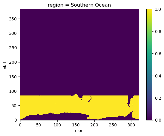
* region (region) <U21 1kB 'Black Sea' 'Baltic Sea' ... 'Hudson Bay'A particular region can be selected by name.
mask3d.sel(region='Southern Ocean').plot();
To visualize all the regions, we can define a help plotting function,
def visualize_mask(mask3d):
    nregion = len(mask3d.region)

    # mask out land
    mask3d = mask3d.where(ds.KMT > 0)

    # visualize the regions
    ncol = int(np.sqrt(nregion))
    nrow = int(nregion / ncol) + min(1, nregion % ncol)

    fig, ax = plt.subplots(nrow, ncol, figsize=(4 * ncol, 3 * nrow), constrained_layout=True)

    for i, region in enumerate(mask3d.region.values):
        plt.axes(ax.ravel()[i])
        mask3d.sel(region=region).plot()

    # delete the unused axes
    for i in range(nregion, ncol * nrow):
        fig.delaxes(ax.ravel()[i])

    fig.suptitle(f'Mask name = {mask3d.mask_name}', fontsize=16)
and apply it to the default mask created above.
visualize_mask(mask3d)

Alternative region masks#
Other useful region masks are pre-defined in the package. list_region_masks returns a list of pre-defined masks.
region_masks = pop_tools.list_region_masks(grid_name)
region_masks
['lat-range-basin', 'Pacific-Indian-Atlantic']
We can visualize all of these using the helper function above.
for region_mask in region_masks:
    mask3d = pop_tools.region_mask_3d(grid_name, mask_name=region_mask)
    visualize_mask(mask3d)


To illustrated how regions cover the global domain, including with overlap, we can sum over the region dimension.
mask3d = pop_tools.region_mask_3d(grid_name, mask_name='lat-range-basin')
mask3d.sum('region').plot();

User defined region masks#
Finally, it is also possible to make a region mask on the fly by building a dictionary containing the defining logic. region_mask_3d accepts a region_defs argument. This is a dictionary of the following form.
region_defs = {region1_name: list_of_criteria_dicts_1,
               region2_name: list_of_criteria_dicts_2,...}
The list_of_criteria_dicts are lists of dictionaries; each must include the keys ‘match’ or ‘bounds’. For instance:
list_of_criteria_dicts_1 = [{'match': {'REGION_MASK': [1, 2, 3, 6]},
                             'bounds': {'TLAT': [-90., -30.]}}]
will return a mask where the default REGION_MASK matches the specified values and TLAT falls between the specified bounds. Multiple entries in the list_of_criteria_dicts are applied with an “or” condition.
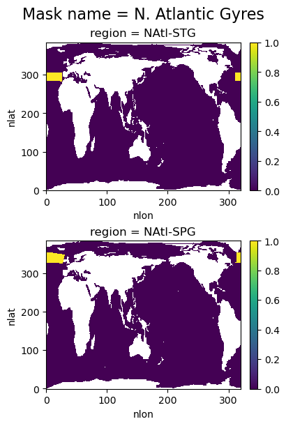
Here’s an example region mask generated for the North Atlantic Subpolar and Subtropical Gyres.
region_defs = {
    'NAtl-STG': [
        {'match': {'REGION_MASK': [6]}, 'bounds': {'TLAT': [32.0, 42.0], 'TLONG': [310.0, 350.0]}}
    ],
    'NAtl-SPG': [
        {'match': {'REGION_MASK': [6]}, 'bounds': {'TLAT': [50.0, 60.0], 'TLONG': [310.0, 350.0]}}
    ],
}

mask3d = pop_tools.region_mask_3d(grid_name, region_defs=region_defs, mask_name='N. Atlantic Gyres')
visualize_mask(mask3d)
%load_ext watermark
%watermark -d -iv -m -g -h
Compiler    : GCC 13.3.0
OS          : Linux
Release     : 6.17.0-1007-aws
Machine     : x86_64
Processor   : x86_64
CPU cores   : 2
Architecture: 64bit

Hostname: build-32095474-project-451810-pop-tools

Git hash: d3177f392237bc6adcac68c1963bdc5fe1a3ccd6

numpy     : 2.0.2
xarray    : 2024.7.0
pop_tools : 0.0.post50+dirty
matplotlib: 3.9.4